Fast-Delivery Performance Metric
The global tide gauge network is an essential component of the global climate observing system, and it is important to develop ways to evaluate the performance of the network. One way to evaluate the global tide network is to test the ability of the network to produce an accurate estimate of global mean sea level (GMSL), which assesses how completely the network samples the global ocean. Sea level variability differs substantially from region to region, and if some areas are not well-sampled, then the error in the global calculation will be larger than if all areas are represented.
Figure 1 shows the UHSLC’s Fast-Delivery Performance Metric, which we define as the spatial sampling error in estimates of GMSL using the UHSLC Fast-Delivery Network. In general, the error decreases in time, which suggests an improving global tide gauge network that more effectively samples the global ocean. It is important to note that the improvement is not only due to adding more gauges to the network, but also better spatial distribution of the gauges to more effectively sample all areas of the global ocean.
Methodology
The performance metric is based on how well the locations sampled by the Fast-Delivery Network can reproduce global mean sea level calculated from satellite altimetry. Here we use the Aviso gridded altimetry product to generate the metric, and we only use Fast-Delivery tide gauge locations that are within 2° of an Aviso grid cell for consistency between the datasets. The tide gauge locations are shown in Figure 2.
We begin by grouping the tide gauge locations into clusters where sea level tends to vary coherently (colors in Figure 2). When we compute the global mean from the tide gauge locations, we first average data in the clusters and then average the clusters. This reduces the effect of over-sampling in some areas where the network is particularly dense. The clusters are defined using an agglomerative hierarchical cluster analysis of the Aviso data (not tide gauge data) from the grid cells closest to each gauge. We use the Aviso time series instead of the tide gauge data, because here we are only interested in the spatial sampling error; i.e., how optimal are the tide gauge locations for sampling the global ocean? Using the tide gauge data itself includes other sources of error (land motion, instrumental error, etc.) that we plan to address in future analysis.
For each time since 1950, we form a global mean of cluster means using Aviso data from ONLY the tide gauge locations that have data at that time. We then calculate the standard deviation of the differences between this global mean time series and the “true” global mean (which is the global mean using the full Aviso grid). This standard deviation is the 1σ sampling error of the tide gauge network configuration at that time. We see that this error decreases in time (Figure 1), which indicates that the Fast-Delivery Network is sampling the ocean more effectively now than in the past.
How has the network improved?
Sampling of the global ocean by the Fast-Delivery tide gauge network has steadily improved since 1950 (Figure 1). In large part, this improvement is due to an increase in the number of tide gauges during that time (Figure 3). However, increasing the number of gauges is only useful insofar as the new tide gauges are not redundant. It is more important to install one new gauge in a previously unsampled region of the ocean than it is to install 10 new gauges where other gauges already exist.
For example, the number of tide gauges in the Fast-Delivery Network decreased from 1995 to 2015 (Figure 3), yet the global mean sampling error of the network continued to fall (Figure 1). We can understand this apparent contradiction by looking at maps of the tide gauge locations with data at those times (Figure 4). The decrease in the number of tide gauges from 1995 to 2015 is in large part due to an abrupt decrease in the number of gauges contributing Fast-Delivery data from coastlines of the Northwest Pacific. There are a number of remaining gauges in that area, however, and the effect of this loss on the global sampling efficacy is small. In contrast, sampling of the Indian Ocean improved considerably during that time. The net affect of these changes is a decrease in the overall number of gauges, but an increase in the ability of the network to capture global change.
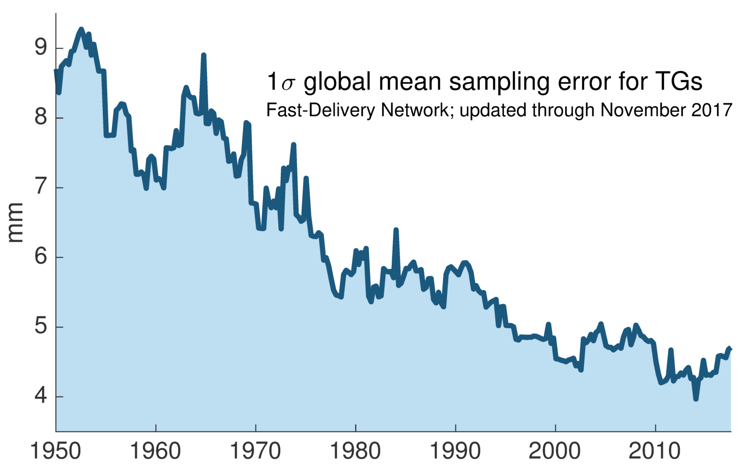
Figure 1: One standard deviation (1σ) sampling error when estimating global mean sea level from Fast-Delivery tide gauges. The sampling error decreases in time as the ability of the Fast-Delivery Network to effectively sample the global ocean improves. The improvement is not only due to increasing the number of gauges, but also improving the spatial distribution of gauges to better sample different areas of the global ocean.

Figure 2: Locations of tide gauges in the Fast-Delivery Network that are within 2º of a grid cell in the Aviso gridded altimetry product. Colors represent clusters of locations where sea level tends to vary coherently. Colors are repeated due to the large number of clusters.
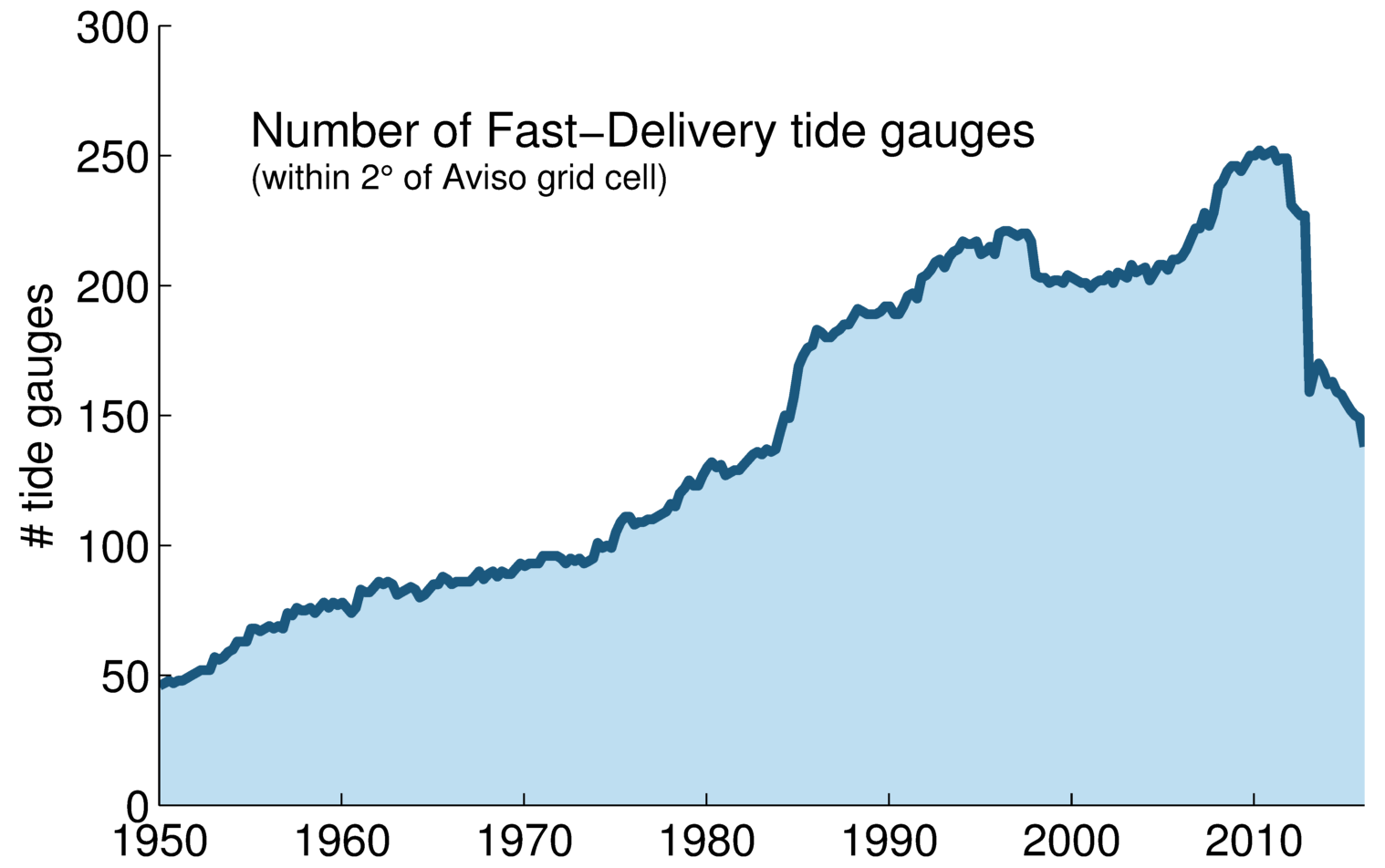
Figure 3: Number of tide gauges in the Fast-Delivery Network (within 2º of an Aviso grid cell) since 1950. The abrupt fall in the number of gauges in recent years is primarily due to a substantial decrease in the number of gauges in the Northwest Pacific contributing Fast-Delivery data.

Figure 4: The Fast-Delivery Network in (a) 1995 and (b) 2015. Note the loss of gauges from 1995 to 2015 in the Northwest Pacific and the addition of gauges across the Indian Ocean.